Compute dt/t
This code is responsible for the calculation of dt/t using the result of the MWCS calculations.
Configuration Parameters
dtt_lag: How is the lag window defined [dynamic]/static (default=static)dtt_v: If dtt_lag=dynamic: what velocity to use to avoid ballistic waves [1.0]km/s (default=1.0)dtt_minlag: If dtt_lag=static: min lag time (default=5.0)dtt_width: Width of the time lag window [30]s (default=30.0)dtt_sides: Which sides to use [both]/left/right (default=both)dtt_mincoh: Minimum coherence on dt measurement, MWCS points with values lower than that will not be used in the WLS (default=0.65)dtt_maxerr: Maximum error on dt measurement, MWCS points with values larger than that will not be used in the WLS (default=0.1)dtt_maxdt: Maximum dt values, MWCS points with values larger than that will not be used in the WLS (default=0.1)
The dt/t is determined as the slope of the delays vs time lags. The slope is calculated a weighted linear regression (WLS) through selected points.
1. The selection of points is first based on the time lag criteria.
The minimum time lag can either be defined absolutely or dynamically.
When dtt_lag is set to “dynamic” in the database, the inter-station distance
is used to determine the minimum time lag. This lag is calculated from the
distance and a velocity configured (dtt_v). The velocity is determined by
the user so that the minlag doesn’t include the ballistic waves. For example,
if ballistic waves are visible with a velocity of 2 km/s, one could configure
dtt_v=1.0.
This way, if stations are located 15 km apart, the minimum lag time will be
set to 15 s. The dtt_width determines the width of the lag window used. A
value of 30.0 means the process will use time lags between 15 and 45 s in the
example above, on both sides if configured (dtt_sides), or only causal or
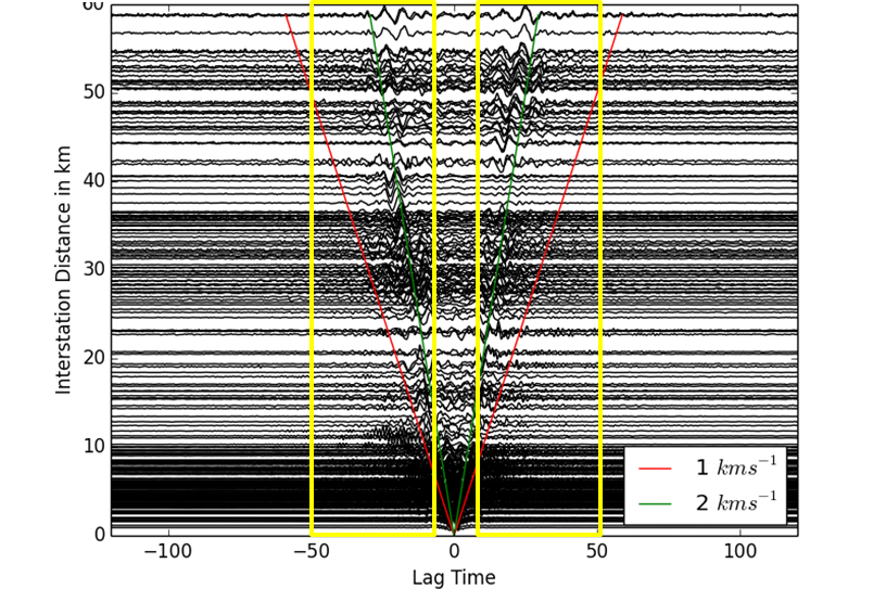
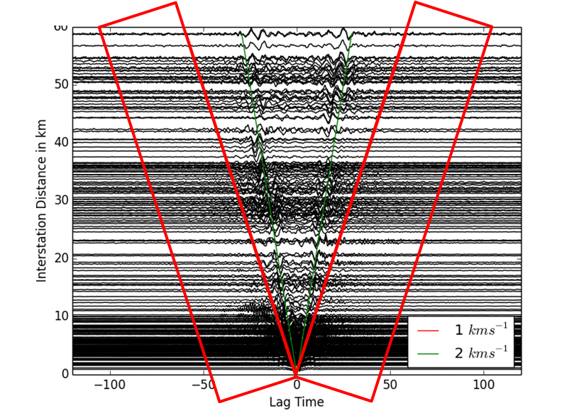
acausal parts of the CCF. The following figure shows the static time lags of
dtt_width = 40s starting at dtt_minlag = 10s and the dynamic time lags
for a dtt_v = 1.0 km/s for the Piton de La Fournaise network (including
stations not on the volcano),
Note
It seems obvious that these parameters are frequency-dependent, but they are currently common for all filters !
Warning
In order to use the dynamic time lags, one has to provide the station coordinates !
2. Using example values above, we chose to use only 15-45 s coda part of the
signal, neglecting direct waves in the 0-15 seconds range. We then select data
which match three other thresholds: dtt_mincoh, dtt_maxerr and
dtt_maxdt.
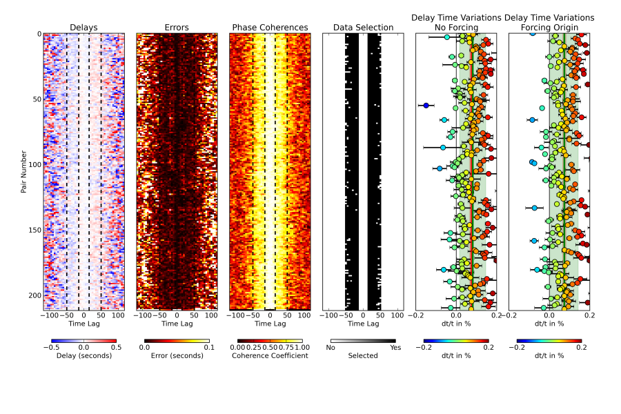
Each of the 4 left subplot of this figure shows a colormapper matrix of which each row corresponds to the data of 1 station pair and each column corresponds to different time lags. The cells are then colored using, from left to right: Delays, Errors, Phase Coherence and Data Selection.
Once data (cells) have been selected, they are analyzed two times: first using a WLS that is forced to pass the origin (0,0) and second when a constant is added to allow for the WLS to be offset from the origin. For each value, the error is computed and stored. M0 and EM0 are the slope and its error for the first WLS, and M, EM together with A and EA are the slope, its error, the constant and its error for the second WLS. The output of this calculation is a table, with one row for each station pair.
Date,          A,        EA,        EM,       EM0,         M,          M0,       Pairs
2013-01-06,-0.1683728,0.0526606,0.00208377,0.00096521, 0.00682021, 0.00037757,BE_GES_BE_HOU
2013-01-06,-0.0080464,0.0577936,0.00291327,0.00097298,-0.00226910,-0.00264354,BE_GES_BE_MEM
2013-01-06, 0.1007472,0.0144648,0.00179566,0.00454172,-0.00145738, 0.00741478,BE_GES_BE_RCHB
2013-01-06,-0.0556811,0.0098926,0.00057839,0.00108102,-0.00328965,-0.00136075,BE_GES_BE_SKQ
2013-01-06, 0.0150866,0.0202243,0.00096543,0.00089832, 0.00083714, 0.00104507,BE_GES_BE_STI
2013-01-06, 0.0268309,0.0328997,0.00153137,0.00150261, 0.00302331, 0.00302451,BE_GES_BE_UCC
2013-01-06,-0.0121293,0.0043351,0.00039019,0.00041347, 0.00025836,-0.00042709,BE_HOU_BE_MEM
2013-01-06, 0.1076247,0.0188662,0.00076824,0.00216383,-0.00030791, 0.00112692,BE_HOU_BE_RCHB
2013-01-06,-0.0468485,0.0194492,0.00069968,0.00078207,-0.00066133, 0.00027102,BE_HOU_BE_SKQ
2013-01-06, 0.0203057,0.0161316,0.00131522,0.00131182, 0.00051626,-3.10306611,BE_HOU_BE_STI
...
2013-01-06,-0.0022588,0.0037141,0.00010340,9.1996e-05, 0.00073635, 0.00076238,ALL
To run this script:
msnoise compute_dtt
Grouping Station Pairs
Although not clearly visible on the figure above, the very last row of the matrix doesn’t contain information about one station pair, but contains a weighted mean of all delays (from all pairs) for each time lag. For each time lag, delays from each pair is taken into account if it satisfies the same criteria as for the individual data selection. Once the last row (the ALL line) has been calculated, it goes through the normal process of the double WLS and is saved to the output file, as visible above. In the future, MSNoise will be able to treat as many groups as the user want, allowing, e.g. a “crater” and a “slopes” groups.
Forcing vs No Forcing through Origin
The reason for allowing the WLS to cross the axis elsewhere than on (0,0) is,
for example, to study the potential clock drifts or noise source position
variations. By default, the msnoise plot dvv plot shows the results
of the `Not Forced WLS.
Mean of All Pairs vs Mean Pair
Warning
the ALL pair is still calculated and output in the DTT files,
but its output is no longer displayed on the graphs. new in 1.6.
The dt/t calculated using the mean pair (ALL, in red on subplots 4 and 5) and by calculating the weighted mean of the dt/t of all pairs (in green) don’t show a significant difference. The standard deviation around the latter is more spread than on the former, but this has to be investigated.