Compute Cross-Correlations
This code is responsible for the computation of the cross-correlation functions.
This script will group jobs marked “T”odo in the database by day and process them using the following scheme. As soon as one day is selected, the corresponding jobs are marked “I”n Progress in the database. This allows running several instances of this script in parallel.
As of MSNoise 1.6, the compute step has been completely rewritten:
The
compute_ccstep has been completely rewritten to make use of 2D arrays holding the data, processing them “in place” for the different steps (FFT, whitening, etc). This results in much more efficient computation. The process slides on time windows and computes the correlations using indexes in a 2D array, therefore avoiding an exponential number of identical operations on data windows.This new code is the default
compute_cc, and it doesn’t allow computing rotated components. For users needingRorTcomponents, there are two options: either use the old code, now namedcompute_cc_rot, or compute the full (6 components actually are enough) tensor using the new code, and rotate the components afterwards. From initial tests, this latter solution is a lot faster than the first, thanks to the new processing in 2D.It is now possible to do the Cross-Correlation (classic “CC”), the Auto- Correlation (“AC”) or the Cross-Components within the same station (“SC”). To achieve this, we removed the ZZ, ZT, etc parameters from the configuration and replaced it with
components_to_computewhich takes a list: e.g. ZZ,ZE,ZN,EZ,EE,EN,NZ,NE,NN for the full non-rotated tensor between stations. Adding components to the newcomponents_to_compute_single_stationwill allow computing the cross-components (SC) or auto-correlation (AC) of each station.The cross-correlation is done on sliding windows on the available data. For each window, if one trace contains a gap, it is eliminated from the computation. This corrects previous errors linked with gaps synchronised in time that lead to perfect sinc autocorrelation functions. The windows should have a duration of at least “2 times the `maxlag`+1” to be computable.
Configuration Parameters
The following parameters (modifiable via `msnoise admin`) are used for
this step:
components_to_compute: List (comma separated) of components to compute between two different stations [ZZ] (default=ZZ)components_to_compute_single_station: List (comma separated) of components within a single station. ZZ would be the autocorrelation of Z component, while ZE or ZN are the cross-components. Defaults to [], no single-station computations are done. (default=) | new in 1.6cc_sampling_rate: Sampling Rate for the CrossCorrelation [20.0] (default=20.0)analysis_duration: Duration of the Analysis (total in seconds : 3600, [86400]) (default=86400)overlap: Amount of overlap between data windows [0:1[ [0.] (default=0.0)maxlag: Maximum lag (in seconds) [120.0] (default=120.)corr_duration: Data windows to correlate (in seconds) [1800.] (default=1800.)windsorizing: Windsorizing at N time RMS , 0 disables windsorizing, -1 enables 1-bit normalization [3] (default=3)resampling_method: Resampling method Decimate/[Lanczos] (default=Lanczos)remove_response: Remove instrument response Y/[N] (default=N)response_format: Remove instrument file format [dataless]/inventory/paz/resp (default=dataless)response_path: Instrument correction file(s) location (path relative to db.ini), defaults to ‘./inventory’, i.e. a subfolder in the current project folder. | All files in that folder will be parsed. (default=inventory)response_prefilt: Remove instrument correction pre-filter (0.005, 0.006, 30.0, 35.0) (default=(0.005, 0.006, 30.0, 35.0))preprocess_lowpass: Preprocessing Low-pass value in Hz [8.0] (default=8.0)preprocess_highpass: Preprocessing High-pass value in Hz [0.01] (default=0.01)preprocess_max_gap: Preprocessing maximum gap length that will be filled by interpolation [10.0] seconds (default=10.0) | new in 1.6preprocess_taper_length: Duration of the taper applied at the beginning and end of trace during the preprocessing, to allow highpassfiltering (default=20.0) | new in 1.6keep_all: Keep all cross-corr (length: corr_duration) [Y]/N (default=N)keep_days: Keep all daily cross-corr [Y]/N (default=Y)stack_method: Stack Method: Linear Mean or Phase Weighted Stack: [linear]/pws (default=linear)pws_timegate: If stack_method=’pws’, width of the smoothing in seconds : 10.0 (default=10.0)pws_power: If stack_method=’pws’, Power of the Weighting: 2.0 (default=2.0)whitening: Whiten Traces before cross-correlation: [A]ll (except for autocorr), [N]one, or only if [C]omponents are different: [A]/N/C (default=A) | new in 1.5whitening_type: Type of spectral whitening function to use: [B]rutal (amplitude to 1.0), divide spectrum by its [PSD]: [B]/PSD. WARNING: only works for compute_cc, not compute_cc_rot, where it will always be [B] (default=B) | new in 1.6hpc: Is MSNoise going to run on an HPC? Y/[N] (default=N) | new in 1.6
Waveform Pre-processing
Pairs are first split and a station list is created. The database is then
queried to get file paths. For each station, all files potentially containing
data for the day are opened. The traces are then merged and split, to obtain
the most continuous chunks possible. The different chunks are then demeaned,
tapered and merged again to a 1-day long trace. If a chunk is not aligned
on the sampling grid (that is, start at a integer times the sample spacing in s)
, the chunk is phase-shifted in the frequency domain. This requires tapering and
fft/ifft. If the gap between two chunks is small, compared to
preprocess_max_gap, the gap is filled with interpolated values.
Larger gaps will not be filled with interpolated values.
Each 1-day long trace is then high-passed (at preprocess_highpass Hz), then
if needed, low-passed (at preprocess_lowpass Hz) and decimated/downsampled.
Decimation/Downsampling are configurable (resampling_method) and users are
advised testing Decimate. One advantage of Downsampling over Decimation is that
it is able to downsample the data by any factor, not only integer factors.
Downsampling is achieved with the ObsPy Lanczos resampler which we tested
against the old scikits.samplerate.
If configured, each 1-day long trace is corrected for its instrument response. Currently, only dataless seed and inventory XML are supported.
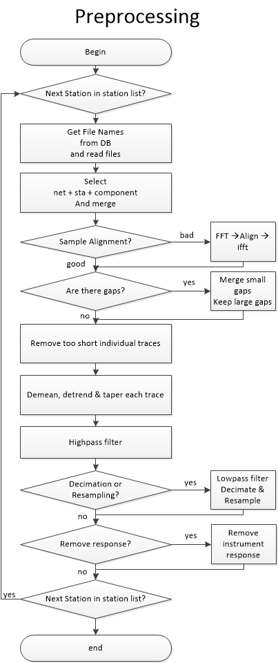
As from MSNoise 1.5, the preprocessing routine is separated from the compute_cc and can be used by plugins with their own parameters. The routine returns a Stream object containing all the traces for all the stations/components.
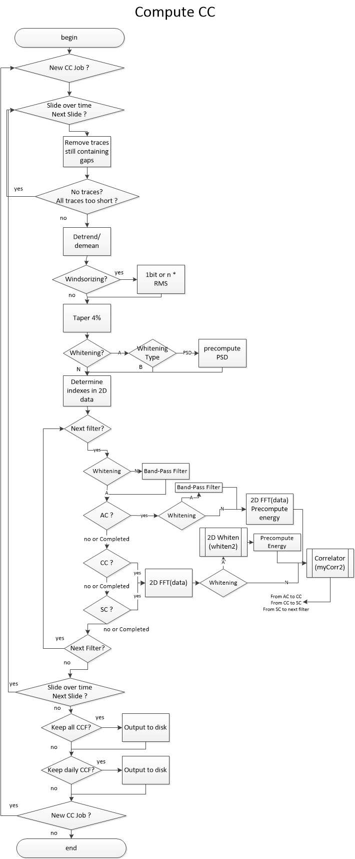
Computing the Cross-Correlations
Processing using msnoise compute_cc
Todo
We still need to describe the workflow in plain text, but the following graph should help you understand how the code is structured
Processing using msnoise compute_cc_rot
Once all traces are preprocessed, station pairs are processed sequentially. If a component different from ZZ is to be computed, the traces are first rotated. This supposes the user has provided the station coordinates in the station table. The rotation is computed for Radial and Transverse components.
Then, for each corr_duration window in the signal, and for each filter
configured in the database, the traces are clipped to windsorizing times
the RMS (or 1-bit converted) and then whitened in the frequency domain
(see whiten) between the frequency bounds. The whitening procedure can be
skipped by setting the whitening configuration to None. The two other
whitening modes are “[A]ll except for auto-correlation” or “Only if
[C]omponents are different”. This allows skipping the whitening when, for
example, computing ZZ components for very close by stations (much closer than
the wavelength sampled), leading to spatial autocorrelation issues.
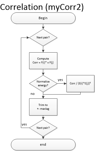
When both traces are ready, the cross-correlation function is computed
(see mycorr). The function returned contains data for time lags
corresponding to maxlag in the acausal (negative lags) and causal
(positive lags) parts.
Saving Results (stacking the daily correlations)
If configured (setting keep_all to ‘Y’), each corr_duration CCF is
saved to the hard disk in the output_folder. By default, the keep_days
setting is set to True and so “N = 1 day / corr_duration” CCF are stacked to
produce a daily cross-correlation function, which is saved to the hard disk in
the STACKS/001_DAYS folder.
Note
Currently, the keep-all data (every CCF) are not used by next steps.
If stack_method is ‘linear’, then a simple mean CCF of all windows is saved
as the daily CCF. On the other hand, if stack_method is ‘pws’, then
all the Phase Weighted Stack (PWS) is computed and saved as the daily CCF. The
PWS is done in two steps: first the mean coherence between the instataneous
phases of all windows is calculated, and eventually serves a weighting factor
on the mean. The smoothness of this weighting array is defined using the
pws_timegate parameter in the configuration. The weighting array is the
power of the mean coherence array. If pws_power is equal to 0, a linear
stack is done (then it’s faster to do set stack_method = ‘linear’). Usual
value is 2.
Warning
PWS is largely untested, not cross-validated. It looks good, but that doesn’t mean a lot, does it? Use with Caution! And if you cross-validate it, please let us know!!
Schimmel, M. and Paulssen H., “Noise reduction and detection of weak, coherent signals through phase-weighted stacks”. Geophysical Journal International 130, 2 (1997): 497-505.
Once done, each job is marked “D”one in the database.
Usage
To run this script:
$ msnoise compute_cc
This step also supports parallel processing/threading:
$ msnoise -t 4 compute_cc
will start 4 instances of the code (after 1 second delay to avoid database conflicts). This works both with SQLite and MySQL but be aware problems could occur with SQLite.
New in version 1.4: The Instrument Response removal & The Phase Weighted Stack & Parallel Processing
New in version 1.5: The Obspy Lanczos resampling method, gives similar results as the scikits.samplerate package, thus removing the requirement for it. This method is defined by default.
New in version 1.5: The preprocessing routine is separated from the compute_cc and can be called by external plugins.
New in version 1.6: The compute_cc has been completely rewritten to be much faster, taking
advantage from 2D FFT computation and in-place array modifications.
The standard compute_cc does process CC, AC and SC in the same code. Only
if users need to compute R and/or T components, they will have to use the
slower previous code, now called compute_cc_rot.