Plotting
MSNoise comes with some default plotting tools.
All plotting commands accept the --outfile argument. If provided, the
figure will be saved to the disk. Names can be explicit, or tell the code to
generate the filename automatically (using the ? question mark), for example:
# automatic naming, save to PNG
msnoise plot dvv -o ?.png

# automatic naming, save to PDF
msnoise plot dvv -o ?.pdf

# explicit naming, save to JPG
msnoise plot dvv -o mydvv.jpg
Customizing Plots
All plots commands can be overridden using a -c argument in front of the plot command !!
Examples:
msnoise -c plot distancemsnoise -c plot ccftime YA.UV02 YA.UV06 -m 5etc.
To make this work, one has to copy the plot script from the msnoise install directory to the project directory (where your db.ini file is located, then edit it to one’s desires. The first thing to edit in the code is the import of the MSNoise API:
from ..api import *
to
from msnoise.api import *
and it should work.
New in version 1.4.
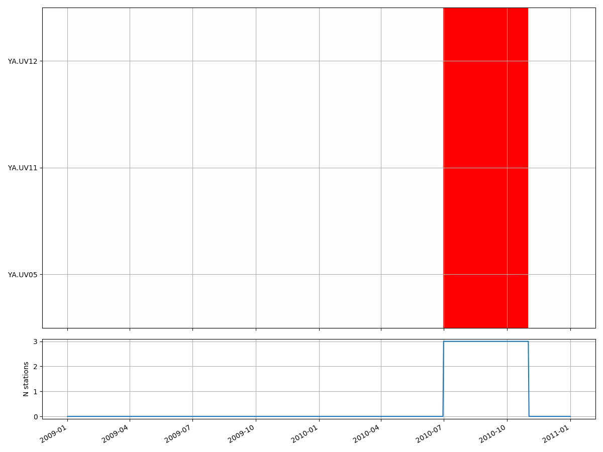
Data Availability Plot
Plots the data availability, as contained in the database. Every day which has a least some data will be coloured in red. Days with no data remain blank.
msnoise plot data_availability --help

Usage:  [OPTIONS]

  Plots the Data Availability vs time

Options:
  -s, --show BOOLEAN  Show interactively?
  -o, --outfile TEXT  Output filename (?=auto)
  --help              Show this message and exit.
Example:
msnoise plot data_availability :
Interferogram Plot
This plot shows the cross-correlation functions (CCF) vs time in a very similar
manner as on the ccftime plot above, but shows an image instead of wiggles.
The parameters allow to plot the daily or the mov-stacked CCF. Filters and
components are selectable too. Passing --refilter allows to bandpass filter
CCFs before plotting (new in 1.5).
msnoise plot interferogram --help

Usage:  [OPTIONS] STA1 STA2 [EXTRA_ARGS]...

  Plots the interferogram between sta1 and sta2 (parses the CCFs)

  STA1 and STA2 must be provided with this format: NET.STA !

Options:
  -f, --filterid INTEGER   Filter ID
  -c, --comp TEXT          Components (ZZ, ZR,...)
  -m, --mov_stack INTEGER  Mov Stack to read from disk
  -s, --show BOOLEAN       Show interactively?
  -o, --outfile TEXT       Output filename (?=auto)
  -r, --refilter TEXT      Refilter CCFs before plotting (e.g. 4:8 for
                           filtering CCFs between 4.0 and 8.0 Hz. This will
                           update the plot title.
  --help                   Show this message and exit.
Example:
msnoise plot interferogram YA.UV06 YA.UV11 -m5 will plot the ZZ component
(default), filter 1 (default) and mov_stack 5:
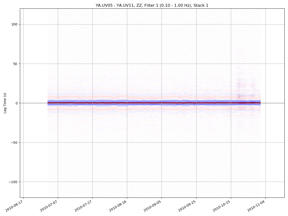
CCF vs Time
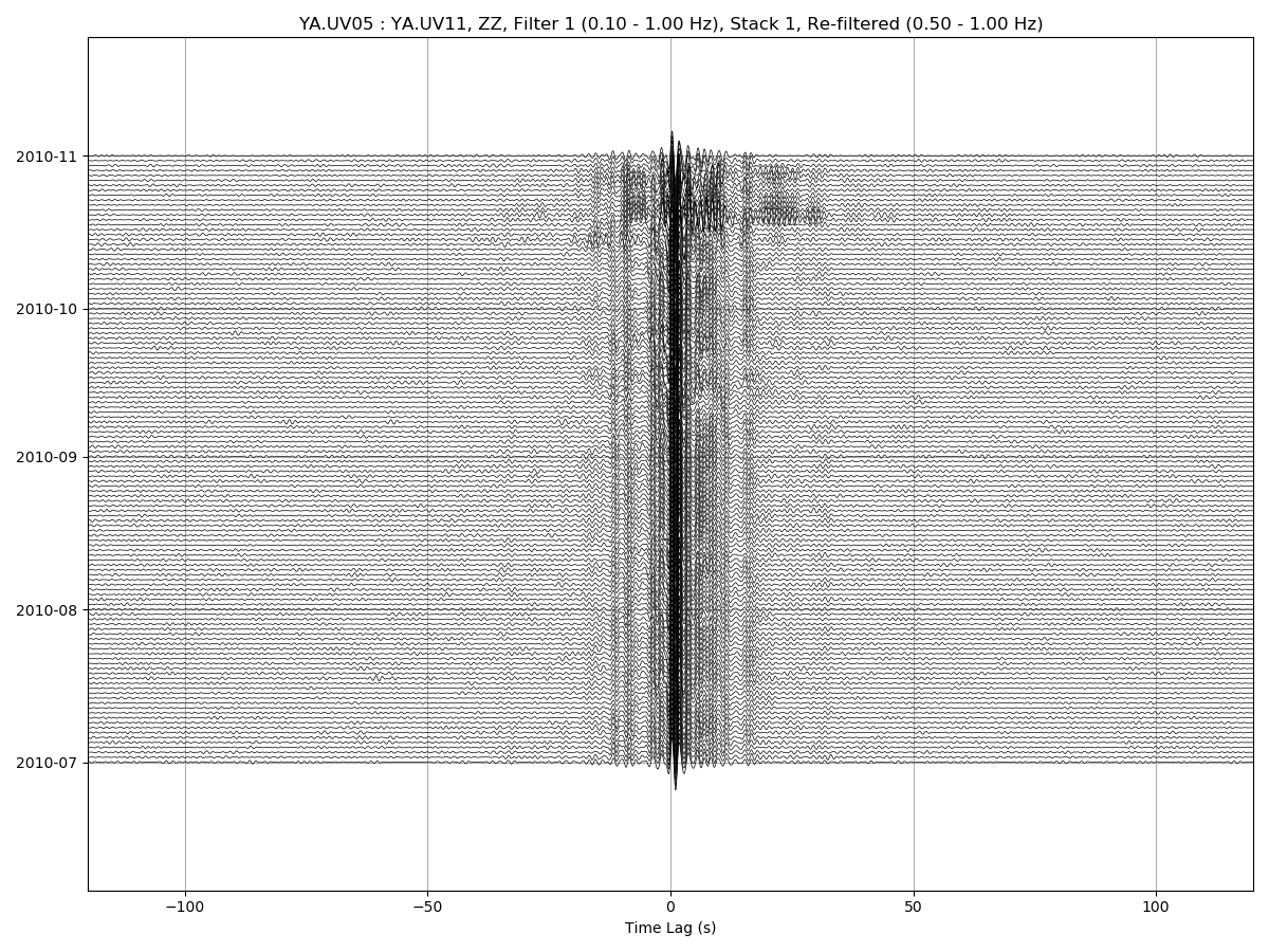
This plot shows the cross-correlation functions (CCF) vs time. The parameters
allow to plot the daily or the mov-stacked CCF. Filters and components are
selectable too. The --ampli argument allows to increase the vertical scale
of the CCFs. The --seismic shows the up-going wiggles with a black-filled
background (very heavy !). Passing --refilter allows to bandpass filter
CCFs before plotting (new in 1.5).
msnoise plot ccftime --help

Usage:  [OPTIONS] STA1 STA2 [EXTRA_ARGS]...

  Plots the ccf vs time between sta1 and sta2

  STA1 and STA2 must be provided with this format: NET.STA !

Options:
  -f, --filterid INTEGER   Filter ID
  -c, --comp TEXT          Components (ZZ, ZR,...)
  -m, --mov_stack INTEGER  Mov Stack to read from disk
  -a, --ampli FLOAT        Amplification
  -S, --seismic            Seismic style
  -s, --show BOOLEAN       Show interactively?
  -o, --outfile TEXT       Output filename (?=auto)
  -e, --envelope           Plot envelope instead of time series
  -r, --refilter TEXT      Refilter CCFs before plotting (e.g. 4:8 for
                           filtering CCFs between 4.0 and 8.0 Hz. This will
                           update the plot title.
  --normalize TEXT
  --help                   Show this message and exit.
Example:
msnoise plot ccftime YA.UV06 YA.UV11 will plot all defaults:
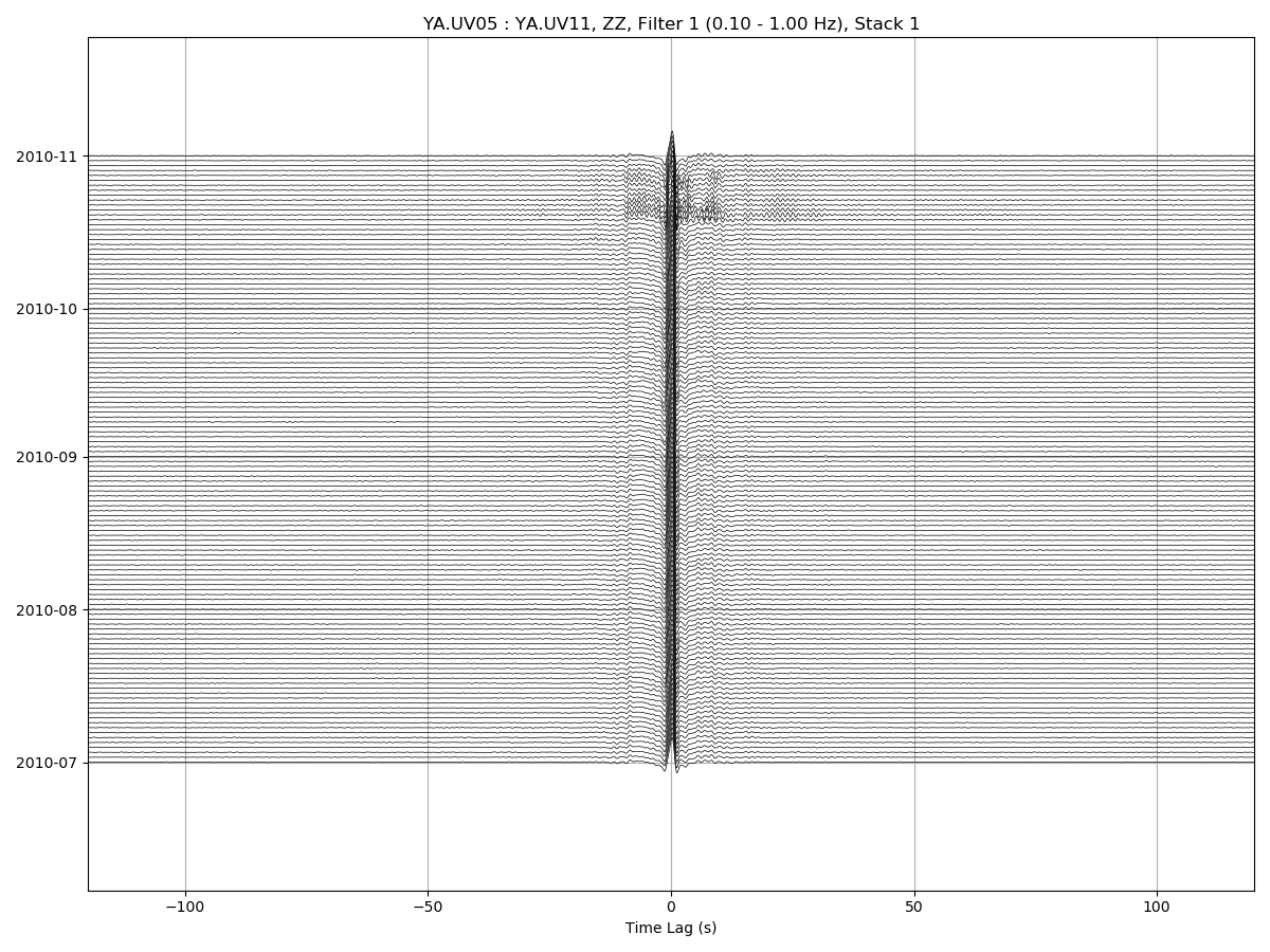
For zooming in the CCFs:
msnoise plot ccftime YA.UV05 YA.UV11 --xlim=-10,10 --ampli=15:
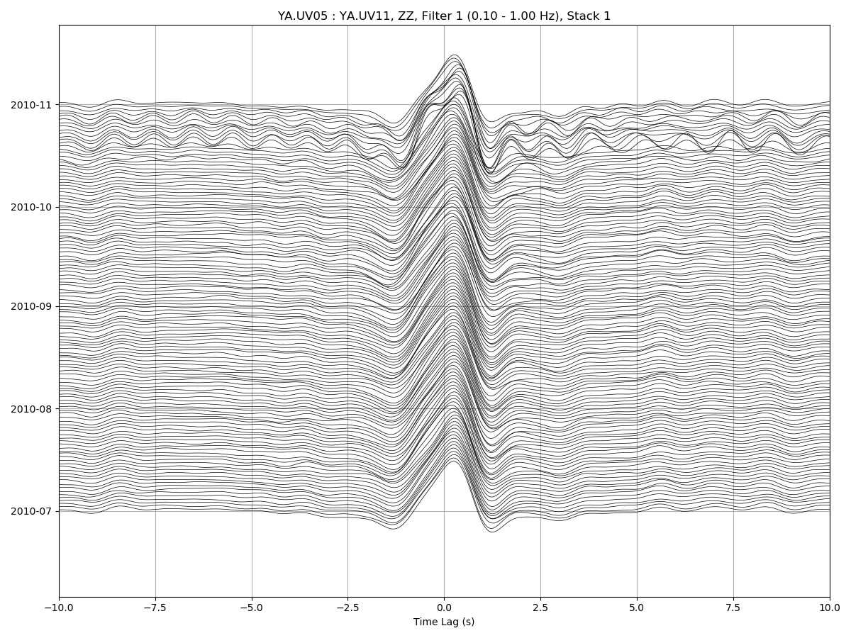
It is sometimes useful to refilter the CCFs on the fly:
msnoise plot ccftime YA.UV05 YA.UV11 -r 0.5:1.0:
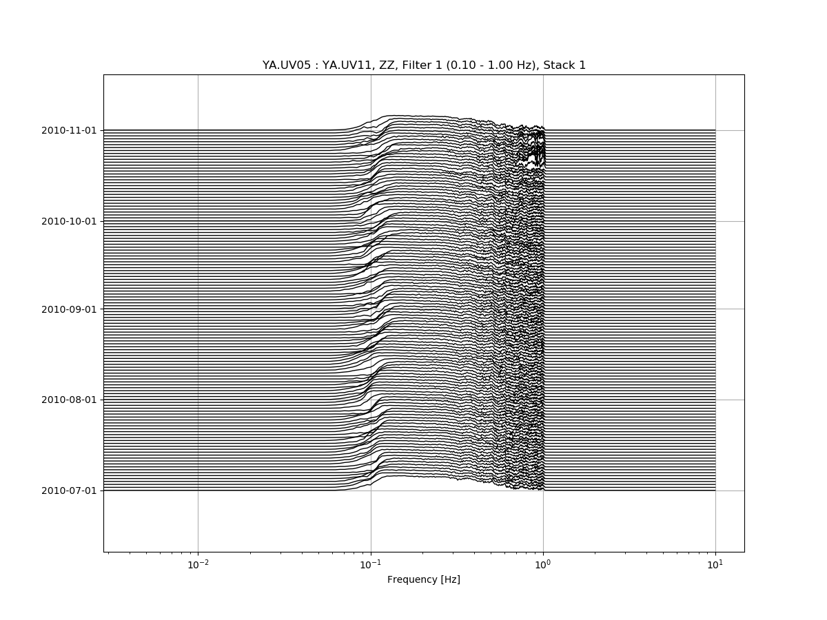
CCF’s spectrum vs Time
This plot shows the cross-correlation functions’ spectrum vs time. The
parameters allow to plot the daily or the mov-stacked CCF. Filters and
components are selectable too. The --ampli argument allows to increase the
vertical scale of the CCFs. Passing --refilter allows to bandpass filter
CCFs before computing the FFT and plotting. Passing --startdate and
--enddate parameters allows to specify which period of data should be
plotted. By default the plot uses dates determined in database.
msnoise plot spectime --help

Usage:  [OPTIONS] STA1 STA2 [EXTRA_ARGS]...

  Plots the ccf's spectrum vs time between sta1 and sta2

  STA1 and STA2 must be provided with this format: NET.STA !

Options:
  -f, --filterid INTEGER   Filter ID
  -c, --comp TEXT          Components (ZZ, ZR,...)
  -m, --mov_stack INTEGER  Mov Stack to read from disk
  -a, --ampli FLOAT        Amplification
  -s, --show BOOLEAN       Show interactively?
  -o, --outfile TEXT       Output filename (?=auto)
  -r, --refilter TEXT      Refilter CCFs before plotting (e.g. 4:8 for
                           filtering CCFs between 4.0 and 8.0 Hz. This will
                           update the plot title.
  --help                   Show this message and exit.
Example:
msnoise plot spectime YA.UV05 YA.UV11 will plot all defaults:
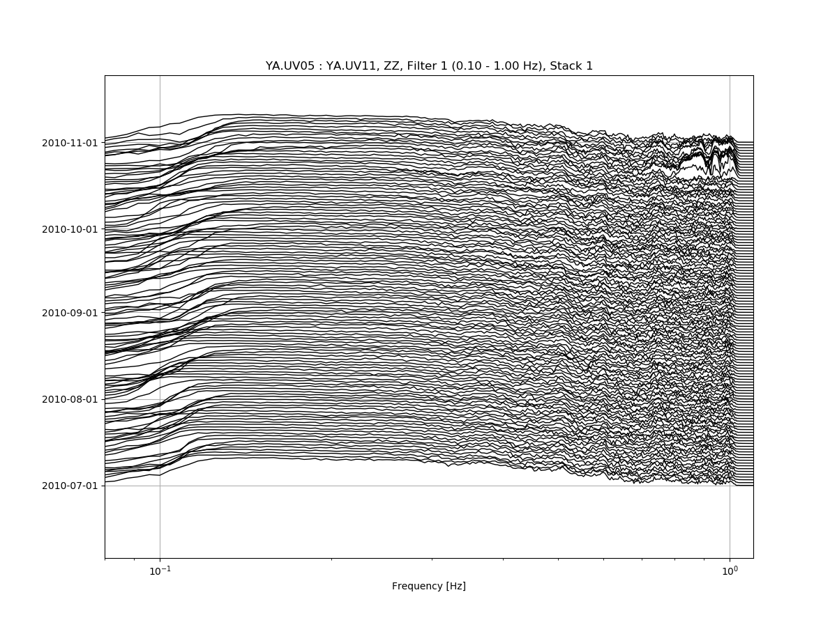
Zooming in the X-axis and playing with the amplitude:
msnoise plot spectime YA.UV05 YA.UV11 --xlim=0.08,1.1 --ampli=10:
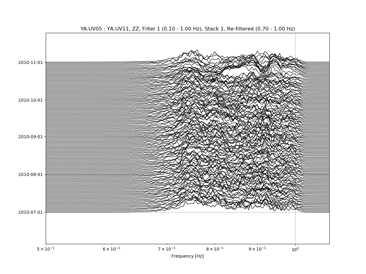
And refiltering to enhance high frequency content:
msnoise plot spectime YA.UV05 YA.UV11 --xlim=0.5,1.1 --ampli=10 -r0.7:1.0:
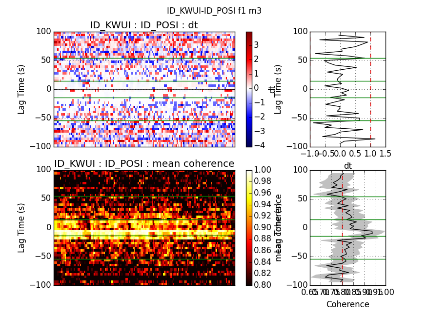
MWCS Plot
This plot shows the result of the MWCS calculations in two superposed images. One is the dt calculated vs time lag and the other one is the coherence. The image is constructed by horizontally stacking the MWCS of different days. The two right panels show the mean and standard deviation per time lag of the whole image. The selected time lags for the dt/t calculation are presented with green horizontal lines, and the minimum coherence or the maximum dt are in red.
The filterid, comp and mov_stack allow filtering the data used.
msnoise plot mwcs --help

Usage:  [OPTIONS] STA1 STA2

  Plots the mwcs results between sta1 and sta2 (parses the CCFs)

  STA1 and STA2 must be provided with this format: NET.STA !

Options:
  -f, --filterid INTEGER   Filter ID
  -c, --comp TEXT          Components (ZZ, ZR,...)
  -m, --mov_stack INTEGER  Mov Stack to read from disk
  -s, --show BOOLEAN       Show interactively?
  -o, --outfile TEXT       Output filename (?=auto)
  --help                   Show this message and exit.
Example:
msnoise plot mwcs ID.KWUI ID.POSI -m 3 will plot all defaults with the
mov_stack = 3:
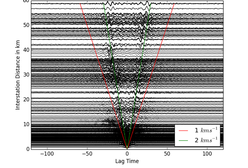
Distance Plot
Plots the REF stacks vs interstation distance. This could help deciding which
parameters to use in the dt/t calculation step. Passing --refilter allows
to bandpass filter CCFs before plotting (new in 1.5). It is also possible to
only draw CCFs for pairs including one station by passing --virtual-pair
followed by the desired NET.STA (new in 1.5).
msnoise plot distance --help

Usage:  [OPTIONS] [EXTRA_ARGS]...

  Plots the REFs of all pairs vs distance

Options:
  -f, --filterid INTEGER  Filter ID
  -c, --comp TEXT         Components (ZZ, ZR,...)
  -a, --ampli FLOAT       Amplification
  -s, --show BOOLEAN      Show interactively?
  -o, --outfile TEXT      Output filename (?=auto)
  -r, --refilter TEXT     Refilter CCFs before plotting (e.g. 4:8 for
                          filtering CCFs between 4.0 and 8.0 Hz. This will
                          update the plot title.
  --virtual-source TEXT   Use only pairs including this station. Format must
                          be NET.STA
  --help                  Show this message and exit.
Example:
msnoise plot distance will plot all defaults:
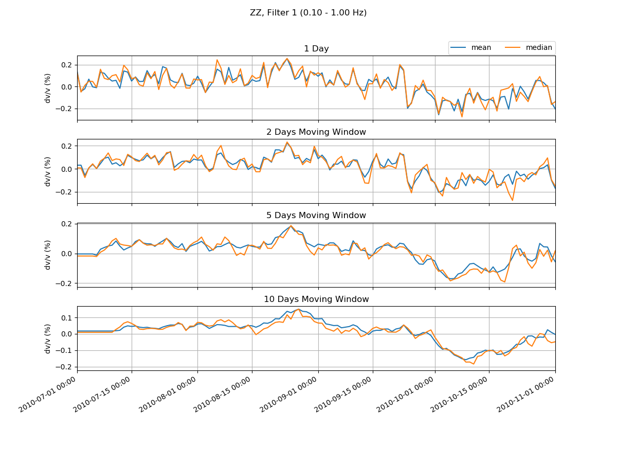
dv/v Plot
This plot shows the final output of MSNoise.
msnoise plot dvv --help

Usage:  [OPTIONS]

  Plots the dv/v (parses the dt/t results)

  Individual pairs can be plotted extra using the -p flag one or more times.

  Example: msnoise plot dvv -p ID_KWUI_ID_POSI

  Example: msnoise plot dvv -p ID_KWUI_ID_POSI -p ID_KWUI_ID_TRWI

  Remember to order stations alphabetically !

Options:
  -f, --filterid INTEGER   Filter ID
  -c, --comp TEXT          Components (ZZ, ZR,...)
  -m, --mov_stack INTEGER  Plot specific mov stacks
  -p, --pair TEXT          Plot a specific pair
  -A, --all                Show the ALL line?
  -M, --dttname TEXT       Plot M or M0?
  -s, --show BOOLEAN       Show interactively?
  -o, --outfile TEXT       Output filename (?=auto)
  --help                   Show this message and exit.
Example:
msnoise plot dvv will plot all defaults:
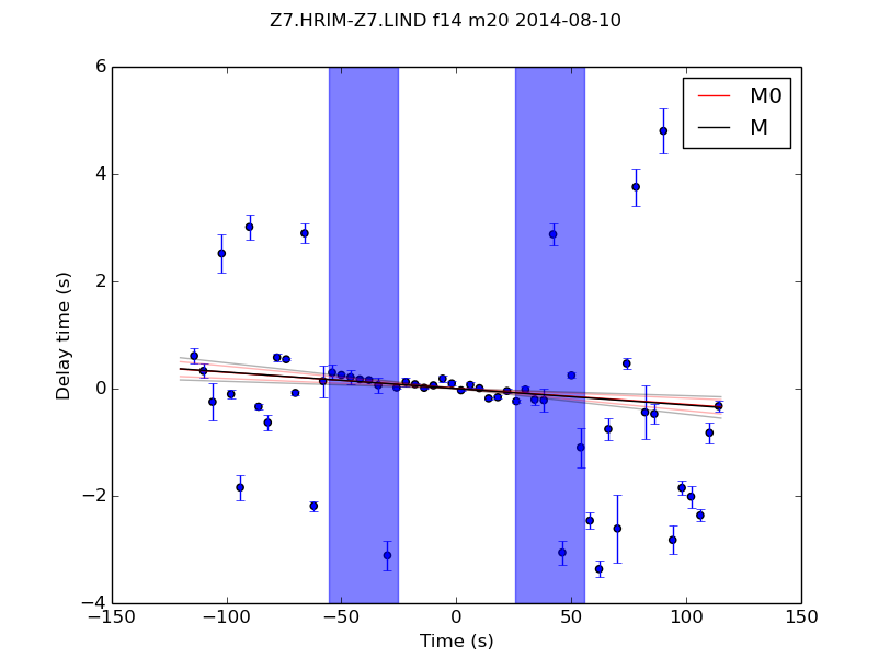
dt/t Plot
This plots dt (delay time) against t (time lag). It shows the results from the MWCS step, plus the calculated regression lines M0 and M. The errors in the regression lines are also plotted as fainter lines. The time lags used to calculate the regression are shown in blue.
msnoise plot dtt --help

Usage:  [OPTIONS] STA1 STA2 DAY

  Plots a graph of dt against t

  STA1 and STA2 must be provided with this format: NET.STA !

  DAY must be provided in the ISO format: YYYY-MM-DD

Options:
  -f, --filterid INTEGER   Filter ID
  -c, --comp TEXT          Components (ZZ, ZR,...)
  -m, --mov_stack INTEGER  Mov Stack to read from disk
  -s, --show BOOLEAN       Show interactively?
  -o, --outfile TEXT       Output filename (?=auto)
  --help                   Show this message and exit.
Example
msnoise plot dtt Z7.HRIM Z7.LIND 2014-08-10 -f 14 -m 20 will plot:
New in version 1.4: (Thanks to C.G. Donaldson)